
When setting up your simulation, you must fill in a probability law defining the task execution time.
The different laws proposed in the Iterop simulation tool are :
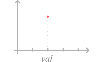
Constant Law
This law represents a constant turnaround time. The time it takes to complete the task will always be the same.
For this law, you need to enter only one value.
Example: the task always takes 5 minutes to complete.
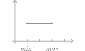
Uniform Law
This law requires two time values min and max. The task will then take a random time between these two values and the probability of a value being drawn is the same regardless of the values.
Example: you define in value min 2 minutes and in value max 20 minutes. During the simulation, the task will take a random value between 2 and 20 minutes.
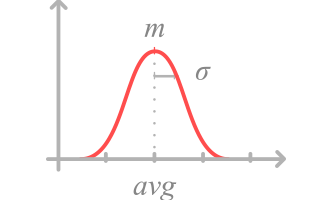
Normal Law
This law requires two parameters: average and standard deviation. The standard deviation represents the drilldown of your data.
To simplify the setting, it is good to know that 99% of the times generated by this law will be between [ mean – 3 standard deviations , mean + 3 standard deviations ].
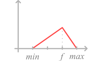
Triangular Law
This law requires three parameters: min, max and mod. The task will most often take the mod time with min and max extremes.
Laws specific to appearances
For instance, two other laws are available:
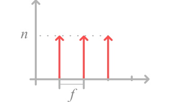
Dirac’s Law
This law requires two parameters: number of instances and frequency.
It consists in starting simultaneously a number of instances of the process, every x frequency. This law is particularly adapted to simulate situations like “A new command is performed every 25 days“.
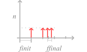
Law by Ramp
This law requires two parameters: initial frequency and final frequency.
Instances will then be created initially every x initial frequency, and this frequency will gradually change until x final frequency is reached.
This is useful for observing how your process reacts to increasing workload, i.e. whether new process instances are launched more and more often.
Act ramps per instance
This law requires three parameters:
- the frequency
- the initial number of executions
- delta.
This law will bring new instances all frequencies. Initially, it will show “initial number of executions” instances, then will show delta more each time.
For example : you have frequency=5min, initial number = 3 and delta = 5, you will have in your simulation 3 instances at t=0, then 8 ( 3+5 ) instances at t=5min, then 13 ( 3+5+5 ) instances at t=10min .
This law also allows you to analyze the scalability of your process, but this time observing the behavior if you have more and more instances.
All together
This law will start as many instances as you want to simulate in the first minute of simulation. If you have chosen to run your simulation over a period of time, you must enter the number of instances to be initiated.

