Configure the simulation of a process

In order to be able to simulate the process, certain information must be filled in. Thus, the n*1 view will allow you to configure your process for modeling.

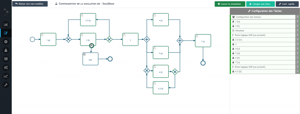
To configure your simulation, you need 3 pieces of information :

• The availability of the actors involved,
• The time it takes to complete each task,
• The probability for logical gates that the process instance follows one branch or another.

Configuration of the actors

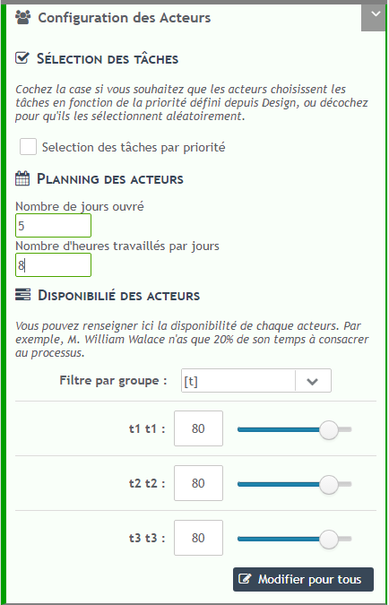
The panel “Configuration of actors” located on the right ( 3 ) allows you to define the availability of your actors. Indeed, it is rare that a user has 100% of his time to devote to the process, so you can define for each actor an availability between 0% and 100%.
If you wish, you can also define an availability for all the actors of the same group, by clicking on button 1.

Task configuration

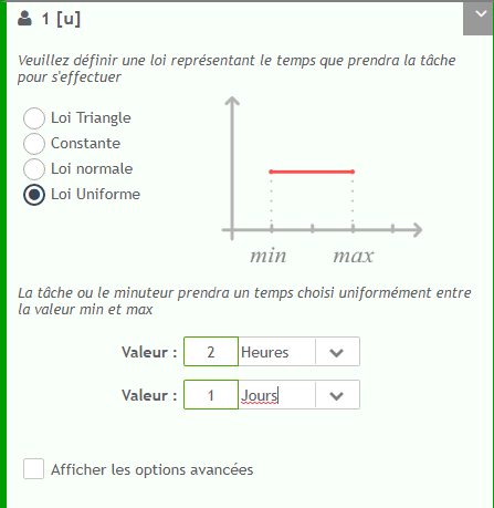
In the panel on the right, you can configure each task and each logical gate. For timers and sub-processes, only one law of probability is required.

Finally, you have to fill in the probabilities of each branch for the logic gates. The question we can ask is “out of 100 files, how many on average go through step ###?”.

Advanced task options

In the task configuration, it is possible to further develop the configuration parameters. You can set :

• Temporary actors to see how your model would behave if you added an actor on certain task.
• The way orders are processed. That is, the order in which the actors handle the tasks to be performed. You have 3 options:
  1. First In First Out (FIFO). This is the default layout, the instances having arrived first on the task are processed first.
  2. First in first out in process (FIFO per process). Priority cases are those that have been in the process the longest.
  3. First in last out (LIFO). This is modeling for a stack of documents, the last one on the stack will be the first to be processed.
• You can also set all the tasks.> of the process in the advanced options section of the quick configuration pane.
• A weakening factor. Some tasks are faster if they are performed for the second time for the same instance. For example, to say that a task is twice as fast on the second pass; you can set a damping factor of 0.5. field of the multiplicative factor> allows you to define the behavior for subsequent passes to the second pass.
  • If this box is ticked, the third run will only take 1/4 of the initial time, the fourth 1/8 .
  • If this box is not checked, all subsequent passages after the first one (for the same instance) will take half of the initial time.

Door configuration

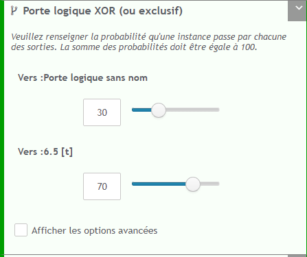
exclusive logic gates must have a probability sum of branches equal to 100%, while inclusive logic gates can have probability sums greater than 100%, reflecting the fact that several paths can be taken at the same time.

Start the simulation

When starting the simulation, you must enter several criteria to test your process.

The configuration of the instances is used to define a law of appearance for process instances. You can define that 10 new instances are created every two hours, or that a new instance is created on average every 3 days. (see Laws of probability).

Define simulation criteria

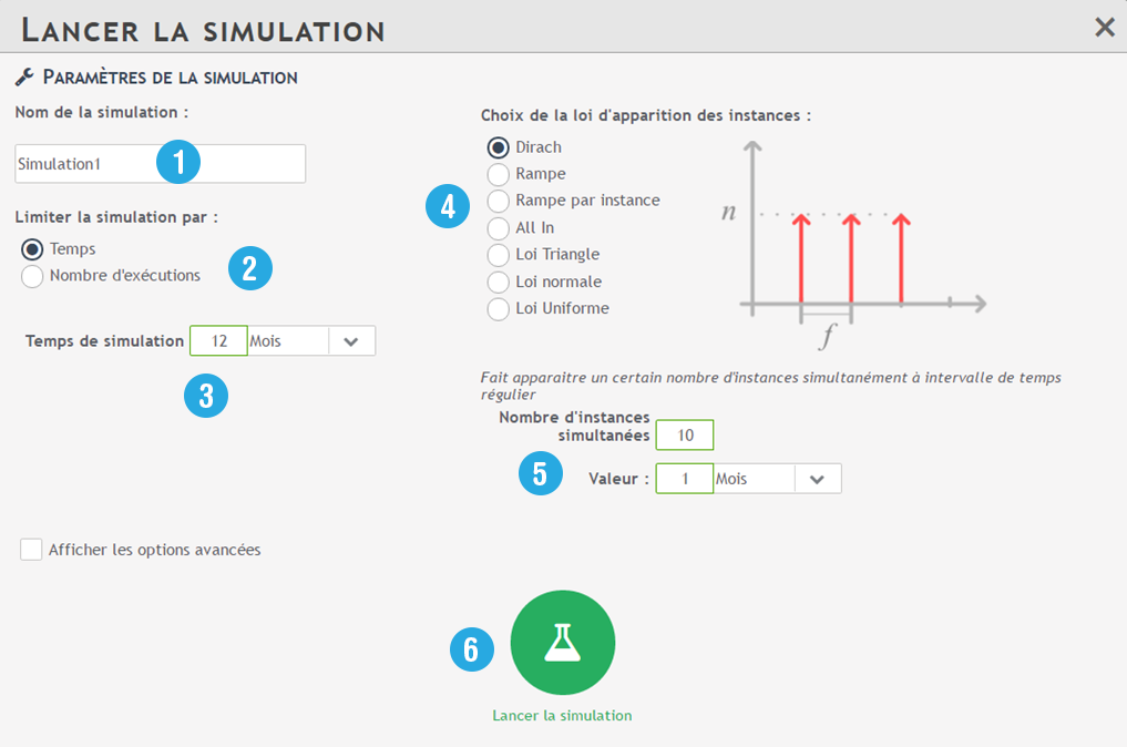
1️⃣ The name of your simulation: the name is automatically filled in by “Simulation”.

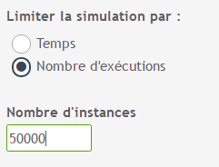
2️⃣ Simulation limitation: you can choose to limit your simulation either by the duration or by the number of executions.

3️⃣ Value : Enter either the simulation time or the desired number of runs.

4️⃣ Choose the law of appearance: see Laws of probability.

5️⃣ Display criteria : you can delimit the simulation with frequency or number of simultaneous launches.

For example: I would like to simulate the customer claim process over 1 year. I estimate that I would have an average of 100 launches per month of this process. I choose Dirach’s law to have these posting criteria.

6️⃣ Start simulation

Advanced options for launching the simulation

You can define a power-on time. In order to have more realistic results, it may be interesting to start simulating your process after a certain period of time, so that it is not empty at the beginning of your simulation. This allows you to define an initial simulation time that will not be taken into account in the results. You can find this ramp-up time either by basing yourself on the laws you have defined for your tasks, or by running an initial simulation and analyzing the process load curve.

• Modify the random number generator : in order to offer you consistent results, the same random number generator is used for each simulation. This means that by running a simulation twice on the same process you will always get the same results. By checking this option, you can decide to modify this random generator to observe different results on the same process.
• Number of simulations : in order to stabilize your results, you may decide to run several simulations simultaneously. The results presented will then be the average of the set of results obtained. Next to these results, you will see numbers in brackets. They represent a range on your value, meaning that about 95% of your results are in the mean +- value range.

This value mathematically represents two standard deviations on your data. It is then more interesting to run 30 simulations of 100 instances than 3 of 1000 instances.